Monday 19 November 2018

Looking inside soot particles

By looking into early soot particles using a high magnification electron microscopes and a "computational microscope" we can start to construct a picture of how the molecules are arranged and better understand how to halt soot formation which is bad for human health and for our planet.

We have recently published two papers that have approached this question from two different directions; Kimberly Bowal leading the charge from the computational side and Dr Maria Botero from the experimental side

Together they provide an interesting picture of how mixtures of aromatic molecules are arranged in liquid soot, carbonise as they are heated in the flame and helps us better understand how to stop soot from forming or provides means of destroy them more readily.

Computational microscope

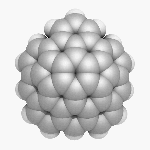
Using accurate mathematical descriptions of the interactions between atoms we can simulate the way molecules self-assemble and see inside a small soot particle. Previously our group has focused only on clusters composed of a single type of molecule. An example of a cluster of coronene is shown below.
Soot is not made up of a single molecule but many hundreds of different sized aromatic molecules. So in this paper, we wanted to study how mixtures of different sized aromatic molecules arrange themselves. There are quite a few challenges simulating such as system;
  1. We can only simulate small isolated clusters otherwise the simulations will take years to compute
  2. We can only simulate for a short duration of simulation time (nanoseconds) but we want to figure out what the most stable arrangement of molecules is over the timescale of soot formation (milliseconds).
The first challenge is problematic as clusters in the flame will be exchanging molecules with the gas phase. This would be too challenging to attempt with such large clusters. Instead we apply a rubber band to molecules that leave the cluster so they always rebound back to the cluster. 

The second challenge is overcome by simulating hundreds of each cluster in parallel all at slightly different temperatures we then exchange clusters that are more ordered with lower temperature clusters. In this way low energy orientations get cooled and quenched providing the most stable arrangement. This method is called replica exchange molecular dynamics and has been used to simulate transformation of cellulose into coals on geological timescales so it is able to really accelerate the whole simulation to flame timescales.

The low temperature structure is also not influenced by the rubber band (as it is a solid so no evaporation occurs on simulation timescales) and therefore we are able to find out given an initial configuration of different sized aromatic molecules what is the most stable cluster geometry. 

Here are the results from two of the low temperature clusters (below). You can see the large aromatics on the inside and the small aromatics on the outside. We found this pattern in all of our clusters studied. Big molecules in the middle small molecules on the outside. 
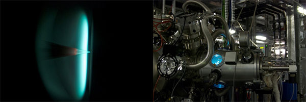

This is also consistent with theory which suggests that the molecules with the greatest interactions would reside in the centre. But what do we see experimentally?

Electron microscope

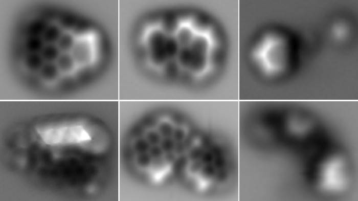
We used an electron microscope which is able to see the aromatic molecules. In order to convert the images into numbers we used a custom program Maria wrote to convert the dark fringes seen in the image below (a) into lines (b) we can then split these lines up and measure how long they are and how curved they are.


Here are some of the many images that Maria collected at each of these heights with the images already converting into lines. Just looking at these fingerprints you can start to see some patterns. The early soot particle contains short fringes (indicating small molecules) while the particles further downstream have long fringes around the outside and smaller fringes inside.


We also found that the fringes in the smallest particles are really quite curved. The fringes suggest that over 60% of the aroamtics at the lowest height above the burner contain pentagonal rings indicating curvature. You can look at a blog post on the impact of these curved aromatic which we published earlier this year.

We also found that at the lowest height you have longer fringes in the middle of the particle compared with the outside. From the computational studies this indicates these early soot cluster are liquid. 

But as you go through the flame this pattern inverts with long fringes around the outside and smaller molecules molecules in the middle. This suggests they are no longer liquid clusters but are now starting to chemically react in the high temperatures (carbonising) and forming longer aromatics when two fuse to become one. This makes sense of recent nanoindentation studies that show that soot that has gone through the entire flame is actually quite hard when you isolate a single soot sphere almost the same hardness as charcoal.

Hypotheses to test

What are planning to do next and how are we going to extend this work
  • We have been talking with other collaborators on using nanoindentation to study early soot particles to confirm if they are indeed liquid. 
  • If we can understand how the carbonisation process occurs we can limit this process. From imaging of soot as they are broken down it was found that the outer shell is the last part to burn away making it important to reduce this can be achieved by lowering the temperature and inhibiting the particles grow too large.
  • We have also been considering clusters of curved molecules and seeing if the same trends of partitioning hold. They certainly look quite different (see below).


So through a combination of computational and experimental studies we have been able to understand how different sized aromatics partition inside soot particles with the arrangement of longer aromatic molecules switching from the inside to the outside of the soot spheres indicating that early on liquid clusters give way to carbonised clusters.

Monday 1 October 2018

Nanotechnology demo using augmented reality


We recently went to the SWITCH technology conference to showcase the different nanomaterials that the chemists in the program make, but how do you show them to people if they are only a few tens of nanometres across. We came up with an augmented reality demo which uses the nyar4psg library in processing allowing for the 3D models of the nanostructures to be picked up and observed in a webcam. 


The business cards on which we printed the visual barcodes for the AR had the material description and link to the academic manuscript printed on the other side of the card. We also had a petri dish with the powder showing the actual material at the macroscale.


By clicking any button on the keyboard it would take a selfie allowing people to take selfies with the nanomaterials which was a lot of fun. Here are some of my favourites.

Monday 3 September 2018

Fingerprinting soot: finding curved aromatics in soot

Fingerprints of molecules in soot particles imaged in an electron microscope showing curved species in the early flame. 
Fingerprinting is a unique way of identifying people by reading off the ridges found on a person's fingers. In a new paper, I and some colleagues used an electron microscope to image the fingerprint of aromatic molecules in early soot particles, finding evidence for a large number of curved molecules, which could be important for reducing soot pollution. Here is a link to the paper or to the open access preprint, "Flexoelectricity and the Formation of Carbon Nanoparticles in Flames". Here is a short video explaining the findings.


Soot emissions cause many deaths around the world while also contributing to global warming, but scientists are still at a loss to explain how soot is formed. We have previously suggested a new mechanism where aromatic molecules curve via pentagon integration and become electrically polarised, interacting strongly with charged species produced in the flame. However, as of yet, no one had measured just how curved (and therefore polar) the molecules are in the early soot particles.

Image result for soot from a ship

To answer this question we imaged the molecules in soot on the nanoscale. To collect some soot we injected a small copper grid covered in amorphous carbon into a flame very similar to a candle. Soot stuck to the amorphous carbon and using an electron microscope we were able to image the molecules in the soot particles sticking to the grid. As you can see in the first image of this post we could convert the dark regions of the image, corresponding to aromatic molecules on their side, into lines. We could determine how many molecules that we imaged indicate pentagonal ring integration and we found this value to be greater than 62.5% of the fringes. This high amount suggests that they are important for soot formation.

We found even in the earliest soot particles sampled at the lowest height, which give us the most insight into soot formation, long fringes 0.9-1.0 nm in length are present (around 15 aromatic rings). We then simulated three curved aromatic molecules of the same length with one, two and three pentagonal rings, providing different amounts of curvature, and computed the tortuosity/curvature. From this analysis, we could conclude that early soot particles (at 10 mm above the flame) have a tortuosity/curvature indicating that two pentagons rings are integrated. Below is a figure of the molecule which corresponds to the average species around 1 nm in width with two pentagonal carbon rings. 


Computing the electric polarisation due to the curved structure, we found a large value of 5.32 debye - around three times that of water, which is substantial. Below is a plot of the electric potential around the molecules introduced earlier.


We found this molecule bound very strongly to charged chemi-ions which are produced in abundance in the flame, using computer simulations. 


The strong interactions of these polar aromatic with chemi-ions need to be explored in more detail as it might help explain many of the electrical effects that have been seen, such as the ability of an electric field to stop soot formation in certain circumstances.


Monday 13 August 2018

37th International Symposium on Combustion


tl;dr >1800 combustion scientists descended on Dublin last week to clean up combustion and pave the way for low carbon fuels. I gave my first talk at an international conference, where we suggested a new mechanism for soot formation based on curved aromatic molecules. 


Over the last week, I have been in Dublin joining with a group of scientists from around the world to better understand combustion. This biannual conference has been going on since 1928 and has a strong community of scientists from universities and industry. 

Why study combustion?

You might be fooled into thinking combustion is a dying field with the world transitioning from fossil fuels to electric transportation. However, this would be too small a view of the field of combustion. In the near future we need to be transitioning our current combustion engines to use low-carbon fuels such as biofuels, hydrogen and perhaps ammonia. This was a large part of the discussion at the conference.  Carbon soot, or particulates from combustion, contribute substantially to global warming and by understanding the formation of soot many hope we will be able to quickly remove this contribution from combustion.

Combustion research doesn't just focus on combustion for transport and heating - surprisingly, many common materials are produced in flames. Car tires are full of very stable carbon particles which are formed in a furnace. These carbon blacks also hold onto the lithium in our batteries allowing us to store electricity in our laptop or cellphone. Practically all of the white titania (titanium dioxide) powder in paint is formed in a flame. The optical fibres that provide us with high-speed internet are made from very pure silica, which can only be produced in a flame. A large part of the symposium was focused on these materials and making new novel materials in flames. 

What happens if we put the flame in there?

I saw talks from people who have put flames in space, super high pressure, vacuum chambers, synchrotrons, high magnetic fields, high voltage electric fields. In this section, I want to show some of the amazing experimental setups and instruments that were presented in talks and posters that are working on understanding soot formation.

Image result for international space station
Image result for Electric-Field Effects on Laminar Diffusion Flames
Flame experiments in space

Flame spray burners using biofuels imaged with lasers [Image Creidt: Kaust]


Atomic force microscopy images of molecules found in soot
Imaging of single soot molecules using atomic force microscopes.
 [Image credit:IBM Research-Zurich and F. Schulz et al./Proc. Combust. Inst.]

Image result for soleil synchrotron
Flame probed with an intense beam of x-rays from a stadium-sized instrument [Image Credit: Soilel]
These new experimental setups are helping us to make leaps and bounds in our understanding of soot formation. Pentagonal rings and radicals were found to be prevalent in aromatic molecules in soot, which were previously thought to contain mainly hexagonal arrangements of carbons and could change the way these molecules self-assemble and react. However, we are still lacking some critical mechanistic understandings of soot formation. 

Soot formation and curved aromatics 

I presented a talk on the mechanism for soot formation and the impact of polar aromatic molecules. I have embedded a copy of the slides below.


We received some excellent questions and suggestions from the community on how to extend these preliminary suggestions in order to test this hypothesis.

An exciting presentation from Francesco Carbone showed evidence that positive ions and not negative ions continue to grow into the soot particles (some of the early work is found in a paper last year), which is what you would expect from the soot nucleation mechanism we are suggesting. 

The great fun of this conference was meeting all of the other researchers from around the world and picking each other's brains over meals and pints of Guinness. Below is a picture of the Kraft research group which was the most numerous we have sent to a combustion symposium so far. Hopefully next symposium two years from now we will be closer to understanding how soot forms and whether these curved molecules contribute.

Tuesday 19 June 2018

Can curved molecules in flames help reduce soot pollution?

Soot is a serious problem which impacts human and the planet's health. The world health organisation estimates that in 2012 seven million people died or 1/8 total deaths around the world, from air pollution with around half from ambient air pollution and the rest from indoor air pollution from cooking on inefficient stoves (WHO). Soot emissions are also the biggest contributor to global warming after the greenhouse gases. So how do we stop soot from forming? The first step is to understand the mechanism by which soot forms, which is surprisingly still not yet fully understood. We have just published an article considering the impact of curved aromatic molecules on the formation mechanism of soot (here is a link to the preprint).

Image result for soot pollution
Credit
So what is currently understood about soot formation? The animation below will aid in illustrating soot formation. It shows the inside of a small lawn mower motor with a transparent plastic engine head allowing for a high-speed camera to capture the combustion inside the engine. 

Credit
A small spark ignites the petrol and air mixture and a blue flame is seen to spread through the cylinder. At the flame front there is enough oxygen and so the fuel burns completely to carbon dioxide and water with the blue colour (the colour is due to excited intermediates C2*, CH* and OH*). However, not all of the flame has enough oxygen to completely combust. Behind the flame front, a build-up of carbon molecules forms soot which glows yellow because it is heated by the combustion. So the yellow colour you see in the figure is soot which is being exhausted into the atmosphere. You can confirm that the yellow colour is from soot at home by placing a metal spoon into the yellow part of the flame and picking up black soot on the spoon.


From the animation inside the engine, you will also have seen the complexity of the flame. To simply the system we often use simple burners to study soot formation which produce very stable candle-like flames (diffusion flame). Below is one of the burners with a schematic to highlight the molecules involved in soot formation. The steps for soot formation are as follows:
  1. Precursor pyrolysis - the fuel breaks down and without enough oxygen a build up of carbon molecules - primarily acetylene occurs.
  2. PAH formation - The acetylene C2H2 reacts through a radical chain reaction into aromatic fused ring molecules.
  3. Inception/nucleation - Small carbon nanoparticle nuclei are formed 
  4. Growth - Some of these nuclei grow to become primary particles tens of nanometres in size.
  5. Aggregation/agglomeration - Primary particles stick together and form fractal-like stringy aggregates.


Step three (inception) is currently the most difficult to understand. Formation of small carbon nanoparticles from aromatic molecules in the flame happens too quickly to be a chemical reaction and must include some physical sticking or clustering to explain the speed of formation. My research group has previously determined that flat PAH (planar aromatics with only hexagonal rings) have been found to not be sticky enough to overcome the high temperatures where soot forms in a flame (~1000-1250°C). This thermal energy shakes the clusters apart.

So what about these curved PAH molecules? It is well known that they are present in soot, corannulene (a simple curved PAH with a pentagon ring surrounded by hexagonal rings) has been extracted from soot and if you decrease the pressure around the flame completely enclosed spherical cages of carbon (fullerenes) can be produced.


corannulene - Wiktionary           Fullerene C60
curved PAH corannulene (left and below click and drag to move the grey model around and zoom with your mouse wheel) and closed cage fullerene (right)


We have previously shown that these molecules contain a large electric polarisation which might be important. So how do these polarised cPAH effect soot formation? In this paper we considered three questions:
  1. What causes lead to curvature and how small do the molecules need to become curved?
  2. Can curved PAH cluster together in the flame where soot forms (~1000-1250°C)?
  3. What other interactions could cPAH have with other precursors (e.g. chemi-ions)?

What causes the curvature and how small do the molecules need to be to curve? Using computational chemistry we could calculate the geometry of lots of different curved aromatic molecules. We found the minimum size is 6 rings to curve a PAH with at least one ring being pentagonal.


It turns out the pentagon containing PAH are planar for larger molecules than you would expect from considering a perfect net of pentagons and hexagons. We found this is due to the bonding of electrons on the top and bottom of the molecule favouring planar geometries which are only overcome when the in-plane bonds are strong enough to pull the molecule into a curved configuration.

Can curved PAH cluster together in the flame where soot forms (~1000-1250°C)? Using another calculation method we worked out how sticky the cPAH are compared with their planar cousins (more negative binding energies means more strongly bound) shown below. Triangles indicate flat PAH and squares indicate cPAH. We found that for one or two pentagons, cPAH have similar binding energies to flat PAH. With three or greater number of pentagons the cPAH bound with less energy than the same sized flat PAH.
We have previously shown that for the size of flat PAH in soot it is unlikely to be able to stablise the small clusters in the soot inception zone. So for cPAH with up to two pentagons, we expect the situation to be similar and with three or more the nucleation is definitely not possible. 

What other interactions could cPAH have with other precursors? In the schematic near the top of the article, we also highlighted some ionic species called chemi-ions (coloured blue). There is a surprising amount of these charges in flames which form from reactions between an excited C-H molecule (which is one of the intermediates that glows blue). When excited CH  reacts with oxygen or acetylene it ejects an electron and becomes positively charged. The impact of these charges can be quite dramatic if you apply an electric field. At a given voltage you can also see the flame conduct electricity with arcs going through the flame. 


Soot formation can also be halted with a strong electric field. The picture below shows with a counterflow burner with fuel from below and air from above. With no electric field applied a yellow sooting flame is found. Applying a strong electric field removes the soot from the flame leaving a blue clean burning flame. This has been explained as charged nuclei and carbon being rapidly sucked out of the flame by the strong electric field.

Top - counterflow diffusion flame without an electric field applied. Bottom - with a strong electric field applied
Credit: Lawton and Weinberg 1969
Curved aromatics are significantly polar and might explain these electrical aspects of soot formation.  The interaction between charge and a dipolar molecule is long range and substantial. The plot below shows a range of curved PAH (covering the range of sizes we see in the flame 10-20 rings) with their binding energy to a charge. To give you a sense of what sort of energies are needed to hold something together at flame temperatures around 165 kJ/mol is usually quoted.


There is quite a lot more work needed to consider this ionic interaction and what impact soot formation here are some of the questions that need answering:
  • How many cPAH are present in early soot nanoparticles?
  • What is the polarity of the cPAH in early soot?
  • Can a cluster of cPAH be stabilised at high temperatures in a flame with a chemi-ion?
  • Is flexoelectricity involved in any other way in soot formation?
So the question Can curved molecules help reduce soot pollution? is yet to be fully answered. We will be presenting these results at the next combustion symposium in Dublin at the end of next month and have more results on the way.

Monday 26 March 2018

Simple Quantum Chemistry: Hartree-Fock in Python

HF-Copy1

Computational chemistry allow properties of molecules to be determined with incredible accuracy. This includes how much energy is stored in a molecule (and how much is released when you combust it), at which frequencies does it vibrate (which can be used to identify chemicals), how quickly a reaction will occur etc. . One of the most widely used method to calculate these properties as a first approximation is the Hartree-Fock (HF) method. Many very successful widely used density functional methods (B3LYP, PBE0, B97) will add in exact exhange calculated using HF to improve the calculation. One of the classic texts in computational chemistry is Modern Quantum Chemistry by Szabo and Ostlund. The book includes a simple calculation of the molecule $HeH^+$ which has the same electronic configuration as the hydrogen molecule but due to the +2 charge on the helium nucleus it is not symmetrical and must be calculated iteratively by converging on a consistent set of parameters which is why the method is often called self consistent field theory (SCF). I have rewritten this example in the python language based on the original Fortran code and try to explain how the calculations are performed and why the operations are done. I have also added in figures to show what the results look like.

Molecular Schrodinger equation

We begin with the time-independent Schrodinger equation for a molecule is

$$H\Psi = E\Psi$$

The Hamiltonian $H$ performs some mathematical operations on the function $\Psi$ and returns a number the energy and the $\Psi$ function unchanged. This equation is what is called a eigenvalue equation and turns out to be fairly straightforward to solve particularly if you make use of matrix algebra which is the method used in with the Roothmaan-Hall equations.

$$\left[ -\sum_i \frac{\nabla_i^{2}}{2} -\sum_A \frac{\nabla_A^{2}}{2} - \sum_{A,i}\frac{Z_{A}}{r_{Ai}}+\sum_{A>B}\frac{Z_A Z_B}{R_{AB}}+\sum_{i>j}\frac{1}{r_{ij}}\right]\Psi(\boldsymbol{r};\boldsymbol{R})=E\Psi(\boldsymbol{r};\boldsymbol{R})$$

or in a more compact form

$$ \left[\hat{T}_e(\boldsymbol{r}) +\hat{T}_N(\boldsymbol{R}) +\hat{V} _{eN}(\boldsymbol{r};\boldsymbol{R})+\hat{V}_{NN}(\boldsymbol{R})+\hat{V}_{ee}(\boldsymbol{r})\right]\Psi(\boldsymbol{r};\boldsymbol{R})=E\Psi(\boldsymbol{r};\boldsymbol{R})$$

You will notice that there are no units because we are making use of atomic units (a.u.) which simplifies the equations by equating these constants to one $m_e=e=h/2\pi=1/(4\pi\epsilon_{0})=1$.

The sums $\Sigma$ have electron $i,j$ and nuclei $A,B$ indices. With the electron positions $\boldsymbol{r}$ and nuclei position $\boldsymbol{R}$ being used to calculate distances between nuclei-electrons $r_{Ai}$, nuclei-nuclei $r_{AB}$ and electron-electron $r_{ij}$. Atomic charges are needed $Z_{A/B}$ in our case $Z_{He}=+2$ and $Z_{H}=+1$.

The terms are, in order;

  • Sum of each electron's kinetic energy $$\hat{T}_e(\boldsymbol{r})=-\sum_i \frac{\nabla_i^{2}}{2}$$
    • Using classical mechanics we can determine the kinetic energy from the velocity $\boldsymbol{v}$ and mass $m$ of the particle (multiplied together to give the momentum $\boldsymbol{p}=m\boldsymbol{v}$) $$E_k=T=\frac{1}{2}m\boldsymbol{v}^2=\frac{\boldsymbol{p}^2}{2m}$$.
    • This classical definition cannot be applied in quantum mechanics as you cannot define a definite position $\boldsymbol{r}$ due to the uncertainity principle which states that the momentum and position cannot be known to any degree of accuracy.
    • We must make use of the quantum mechanical momentum operator $\hat{p} =-i\hbar\nabla$ which comes from the wave description of a free particle. $$T_e = \frac{\boldsymbol{p}^2}{2m} = \frac{(-i\hbar\nabla)^2}{2m} = -\frac{\hbar^2}{2m}\nabla^2$$ ($\nabla$ is the symbol used to specify derivatives in multivariable calculus. i.e $\partial /\partial x$)
    • Think of this as a kinetic energy pressure which due to quantum uncertainity holds the electron away from the nuclei allowing it not to collapse to the positive nuclei.
    • This fluctuation is dependent inversely on the mass so the fluctuation in the light electron is much larger than the heavy nuclei which means it is only neccessary (in most cases) to consider the qunatum mechanical fluctutations of the electrons around fixed nuclei.
  • Sum of each nuclei's kinetic energy $$\hat{T}_N(\boldsymbol{R})=-\sum_A \frac{\nabla_A^{2}}{2}$$
    • Just as the electron does not have a definitive position so also the nuclei do not.
    • The uncertainity of the electron is much greater than the uncertainty of the nuclei due to the much greater mass of the later that we often will ignore the quantum uncertainity in the nuclei.
    • However, for light nuclei such as hydrogen this is important and can lead to interesting quantum tunneling effects.
  • Sum of energy from nuclei-electron attraction $$\hat{V} _{eN}(\boldsymbol{r};\boldsymbol{R})= - \sum_{A,i}\frac{Z_{A}}{r_{Ai}}$$
    • this is an attractive energy between nuclei and electrons and is just coulombs law which is usually written $E_{Coulomb} = \frac{q_A q_B}{4\pi \epsilon_0R_{AB}}$ with two charge $q_A$ and $q_B$ a distance apart $R_{AB}$
    • remember atomic units removes the $4\pi\epsilon_0$ constants, where $\epsilon_0$ is the electric permittivity.
  • Sum of energy from nuclei-nuclei repulsion $$\hat{V}_{NN}(\boldsymbol{R})=+\sum_{A>B}\frac{Z_A Z_B}{R_{AB}}$$
    • a repulsive term this is just coulombs law usually written $E_{Coulomb} = \frac{q_A q_B}{4\pi \epsilon_0R_{AB}}$ with two nuclear charges $q_A$ and $q_B$ a distance $R_{AB}$ apart
  • Sum of electron-electron repulsion $$\hat{V}_{ee}(\boldsymbol{r})=+\sum_{i>j}\frac{1}{r_{ij}}$$
    • electron-electron repulsion similar to the electrostatic term between the nuclei and electrons.

Most often, however, we only consider the electronic problem for a given set of nuclear positions $\boldsymbol{R}$ as the electrons are significantly lighter and therefore can be considered to instantanously adjust for any nuclear position. (However, the energy here does not include the nuclear repulsions which need to be added at the end to get the total energy.)

$$\left[ \hat{T}_e(\boldsymbol{r})+ \hat{V} _{eN}(\boldsymbol{r};\boldsymbol{R})+\hat{V}_{ee}(\boldsymbol{r})\right]\Psi(\boldsymbol{r})=E_{el}\Psi(\boldsymbol{r})$$

Hartree-Fock equation

One of the challenges in solving this equation is that you do not know where the electron resides only where it is statisically likely to be if you took a measurement - called the many-body effect. This makes the terms involving the electron repulsions ($+\sum_{i>j}\frac{1}{r_{ij}}$) difficult to calculate.

In the Hartree-Fock approach the first approximation used is to treat each electron separately interacting with an averaged distribution of the other electrons (mean field approach).

$$\left[ -\sum_i \frac{\nabla_i^{2}}{2}- \sum_{A,i}\frac{Z_{A}}{r_{Ai}}+v_{HF}(i)\right]\Psi(\boldsymbol{r})=\epsilon_{ij}\Psi(\boldsymbol{r})$$

The functions chosen to represent each electron is based on the hydrogen atomic solutions, which are exact, for an electron around an atom of hydrogen the atomic orbitals.

So we consider a product of one-electron wavefunctions $\psi_i(\boldsymbol{r})$ interacting with a mean field of all the other electrons. $$\Psi(\boldsymbol{r}) = \psi_1(\boldsymbol{r}_1)\psi_2(\boldsymbol{r}_2)\psi_3(\boldsymbol{r}_3)...=\prod_i \psi_i(\boldsymbol{r}_i)$$

However this does not have the correct symmetry requirements which means if you swap electrons the sign of the wavefunction inverts. This requirement means that the Fermions (electrons) cannot occupy the same quantum states and do not collapse towards the nucleus. We can construct something called a slater determinant which does have the correct symmetry properties.

$$\Psi(\mathbf{r}_1, \mathbf{r}_2, \ldots, \mathbf{r}_N) = \frac{1}{\sqrt{N!}} \left| \begin{matrix} \psi_1(\mathbf{r}_1) & \psi_2(\mathbf{r}_1) & \cdots & \psi_N(\mathbf{r}_1) \\ \psi_1(\mathbf{r}_2) & \psi_2(\mathbf{r}_2) & \cdots & \psi_N(\mathbf{r}_2) \\ \vdots & \vdots & \ddots & \vdots \\ \psi_1(\mathbf{r}_N) & \psi_2(\mathbf{r}_N) & \cdots & \psi_N(\mathbf{r}_N) \end{matrix} \right|\equiv \left|\psi _1,\psi _2,\cdots ,\psi _N\right.\rangle$$

$\left|\psi _1,\psi _2,\cdots ,\psi _N\right.\rangle $ is often written simply as $\psi_i(\boldsymbol{r}_i)$

This means we can write a set of $i$ equations which can be solved for a set of one-electron wavefunctions.

$$\left[ -\sum_i \frac{\nabla_i^{2}}{2}- \sum_{A,i}\frac{Z_{A}}{r_{Ai}}+v_{HF}(i)\right]\psi_i(\boldsymbol{r}_i)=\epsilon_{ij}\psi_i(\boldsymbol{r}_i)$$

What then is $v_{HF}(i)$ we can consider two interactions a coulomb interaction $\mathscr{J}$ (repulsion between the "averaged out" one-electron orbitals) and an exchange interactions $\mathscr{K}$ which is not classical and is due to electrons of the same spin being indistinguishable which lowers the energy of the system.

$$ v_{HF}(i) = \sum_j \left[ 2\mathscr{J}_j - \mathscr{K}_j\right] $$

Where the sum is over all of the other $j$ electrons. There is a double contribution from the coulomb operator as we are considering closed shell systems where there are two electrons per orbital but the exhange operator is only considered once as this interaction can only be between electrons with like-spins. This means for our HeH+ system it will not contribute as we have

$$ \mathscr{J}_j = \int \psi_j(\boldsymbol{r}_j)^* \frac{1}{r_{i,j}}\psi_j(\boldsymbol{r}_j) dr$$$$ \mathscr{K}_j\psi_i(\boldsymbol{r}_i) = \left[\int \psi_j(\boldsymbol{r}_j)^* \frac{1}{r_{i,j}}\psi_i(\boldsymbol{r}_i)dr\right]\psi_j(\boldsymbol{r}_j) $$

You will notice the indices have switched for the exchange operator.

The first two terms are often considered as the core terms as they are the kinetic energy and potential energy for an isolated system such as the hydrogen atom and therefore they are refered to as $\mathscr{H}^{CORE}$

$$ \mathscr{H}^{CORE} = -\sum_i \frac{\nabla_i^{2}}{2}- \sum_{A,i}\frac{Z_{A}}{r_{Ai}} $$

Putting this all together we get the Hartree-Fock equation

$$ \left( \mathscr{H}^{CORE} + \sum_j \left[ 2\mathscr{J}_j - \mathscr{K}_j\right] \right)\psi_i(\boldsymbol{r}_i) = \sum_j \epsilon_{ij}\psi_i(\boldsymbol{r}_i) $$

Or simply

$$ \mathscr{f}_i\psi_i(\boldsymbol{r}_i) = \epsilon_{i}\psi_i(\boldsymbol{r}_i) $$

where $\mathscr{f}_i$ are the fock operators

Orbitals

The most successful method to construct these one-electron wavefunctions $\psi_i$ is to consider them delocalised over the whole molecule. Therefore there will be a set of orbitals, one for each electron, which are spread over the whole molecule. We call this type of treatment molecular orbital theory. The question then is what functions do we use to treat these one-electron delocalised orbitals. We know the solutions exactly for a hydrogen like atom so we can use atomic orbitals $\phi_i(\boldsymbol{r}_i)$ centred at each atom $\boldsymbol{r}_i$ to be the basis for our delocalised molecular orbitals. We need to be able to optimise the amounts of each of these atomic orbitals in each of our one-electron delocalised orbitals so we consider a linear combination of atomic orbitals (LCAO).

$$\psi_i(\boldsymbol{r}_i) = \sum_{\mu} c_{\mu} \phi_{\mu}(\boldsymbol{r}_i)$$

where the constants $c_i$ are going to be optimised to minimise the energy.

The method relies on the vartionial principle which is true for the Hartree-Fock equations which is that any approximation you make (i.e. describing the electrons as a LCAO) will raise the energy above the real energy of the system. The advantage of a variational method is that you can systematically improve the wavefunction and improve your result knowing that you will be able to converge upon a value (which will be above the actual energy).

The atomic orbitals are called the slater type orbitals for the 1s orbital this can be written as

$$ \phi^{SLA}\left( \boldsymbol{r}\right) = \left( \zeta^3/\pi \right)^{1/2}e^{-\zeta \boldsymbol{r}} $$

Let's have a look at the function by plotting it.

In [1]:
# Need to import some libraries to have the maths functions and plotting
import numpy as np
import scipy.special as sp
import matplotlib.pyplot as plt
%matplotlib notebook # Allows plotting in the notebook

x = np.linspace(-5,5,num=1000)
r = abs(x)

zeta = 1.0

psi_STO = (zeta**3/np.pi)**(0.5)*np.exp(-zeta*r)

plt.figure(figsize=(4,3))
plt.plot(x,psi_STO)
Out[1]:
[<matplotlib.lines.Line2D at 0x1065af0b8>]

Slater type orbitals (STO) are the exact solutions for the hydrogen atom and provide an accurate basis set for many electron molecules however the calculations of the integrals are expensive as their is no simple exact solution for the integrals. One way around this is to approximate the Slater type orbitals using a sum of contracted Gaussian functions (CGF). There are simple analytical expressions for the integrals between two Gaussians so this can save a lot of computing time. Let's look at this for the case of the 1s orbital

$$\phi^{GF}(\alpha)=(2\alpha/\pi)^{3/4}exp(-\alpha r^{2}) $$$$\phi^{CGF}\left( \boldsymbol{r}\right) = \sum_n d_n\phi^{GF}_n(\alpha)$$

We will make use of three Gaussians to approximate the slater type orbitals.

$$\phi^{CGF}_{STO-3G}\left( \boldsymbol{r}\right) = \sum^3_n d_n\phi^{GF}_n(\alpha)$$
In [19]:
# Coeff is the d_n variable in the equation above
Coeff = np.array([[1.00000,0.0000000,0.000000],
                  [0.678914,0.430129,0.000000],
                  [0.444635,0.535328,0.154329]])

# Expon is the alpha variable in the equation above
Expon = np.array([[0.270950,0.000000,0.000000],
                  [0.151623,0.851819,0.000000],
                  [0.109818,0.405771,2.227660]]) 

psi_CGF_STO1G = Coeff[0,0]*(2*Expon[0,0]/np.pi)**(0.75)*np.exp(-Expon[0,0]*r**2)
psi_CGF_STO2G = Coeff[1,0]*(2*Expon[1,0]/np.pi)**(0.75)*np.exp(-Expon[1,0]*r**2) \
                + Coeff[1,1]*(2*Expon[1,1]/np.pi)**(0.75)*np.exp(-Expon[1,1]*r**2) \
                + Coeff[1,2]*(2*Expon[1,2]/np.pi)**(0.75)*np.exp(-Expon[1,2]*r**2)
psi_CGF_STO3G = Coeff[2,0]*(2*Expon[2,0]/np.pi)**(0.75)*np.exp(-Expon[2,0]*r**2) \
                + Coeff[2,1]*(2*Expon[2,1]/np.pi)**(0.75)*np.exp(-Expon[2,1]*r**2) \
                + Coeff[2,2]*(2*Expon[2,2]/np.pi)**(0.75)*np.exp(-Expon[2,2]*r**2)
    
# Plot the three functions
plt.figure(figsize=(5,3))
plt.title("Approximations to a STO with CGF")
plt.plot(x,psi_STO,label="STO")
plt.plot(x,psi_CGF_STO1G,label="STO-1G")
plt.legend()
plt.figure(figsize=(5,3))
plt.plot(x,psi_STO,label="STO")
plt.plot(x,psi_CGF_STO2G,label="STO-2G")
plt.legend()
plt.figure(figsize=(5,3))
plt.plot(x,psi_STO,label="STO")
plt.plot(x,psi_CGF_STO3G,label="STO-3G")
plt.legend()
Out[19]:
<matplotlib.legend.Legend at 0x106ddda58>

As the number of Gaussians is increased the function more closely describes the slater type orbitals. You will also see that nearest the centre (x=0) the approximation is poorest. This region is called the cusp.

We will use this very poor basis set for our HeH+ molecule for ease of calculation but for accurate calculations at the very least a 6-311G(d,p) basis set will used which would have 6 contracted Gaussian functions to describe hydrogen and helium 1s orbital.

Roothaan-Hall equations

The Hartree-Fock equations need to be converted into a tabular form (matrix form) using the basis set of atomic orbitals to allow for a solution to be determined using the computer. We insert our basis set of orbitals $\sum_i c_i \phi^{CGF}_i(\boldsymbol{r}_i)$ (we will drop the superscript and just have the orbitals denoted as $\phi_i$) We are also going to be building up a table by combining different basis set indices so will use the subscripts $\nu$ and $\mu$ to denotes the indices as we build up the table/matrix. We will also replace $(\boldsymbol{r}_\nu)$ with $(1)$ for ease of reading.

$$ \mathscr{f}_i\psi_i(\boldsymbol{r}_i) = \epsilon_{i}\psi_i(\boldsymbol{r}_i) $$$$ \mathscr{f}_i\sum^K_{\nu =1} c_{\nu 1} \phi_{\nu}(1) = \epsilon_{i}\sum^K_{\nu =1} c_{\nu i} \phi_{\nu}(1) $$

We left multiply the other basis set index of our table and integrate.

$$ \sum^K_{\nu =1}c_{\nu 1} \int d\nu_1 \phi_{\mu}(1) \mathscr{f}_i \phi_{\nu}(1) = \epsilon_{i}\sum^K_{\nu =1} c_{\nu i}\int d\nu_1 \phi_{\mu}(1)\phi_{\nu}(1) $$

This last term $\int d\nu_1 \phi_{\mu}(1)\phi_{\nu}(1)$ is called the overlap integral written as $S_{\mu \nu}$. This term will help to illustrate the population of a table if we want to know how much the 1s orbital on the He interacts with the 1s orbital on the H atom we would calculate the values on the diagonal of the overlap matrix (for our calculation below this is 0.45077041 in the code the variable is called S12). However, the overlap of the basis function with itself is one by definition.

$$S_{\mu \nu}= \left[ \begin{matrix} 1.0 & 0.45077041 \\ 0.45077041 & 1.0 \end{matrix}\right] $$

We have another matrix called the Fock matrix $F_{\mu \nu}$ which is made up of the core contributions $\mathscr{H}^{CORE}$ and the effective potential $v_{HF}$ lets see how the matrices are constructed from these.

$$ \int d\nu_1 \phi_{\mu}(1)\mathscr{H}^{CORE}\phi_{\nu}(1) = \int d\nu_1 \phi_{\mu}(1)\left[ -\sum_i \frac{\nabla_i^{2}}{2}- \sum_{A,i}\frac{Z_{A}}{r_{Ai}} \right]\phi_{\nu}(1) = H^{CORE}_{\mu \nu} $$

Where $H^{CORE}_{\mu \nu}$ is another matrix that has to be calculated containing a kinetic energy and potential energy contribution. These are called one electron integrals (as they are the interactions of a single electron in a molecular orbital). In the code the core contributions are broken up into kinetic terms (T11, T12 and T22, note we do not need T21 as the matrix is symmetrical) and potential terms (V11A, V12A, V22A for atom one and V11B, V12B, V22B for the second atom, note the sum is also over the nuclei for this term)

The effective Hartree potential is a bit tricker to calculate.

$$ \int d\nu_1 \phi_{\mu}(1)v_{HF}\phi_{\nu}(1) = \sum_{j=1}^{N/2}\int d\nu_1 \phi_{\mu}(1)\left[ 2\mathscr{J}_j - \mathscr{K}_j \right]\phi_{\nu}(1) = G^{2e}_{\mu \nu \lambda \sigma} $$

Where $N$ is the total number of electrons and for closed shell molecules we want half of these electrons, due to two electrons residing in each occupied molecular orbital. This integrate is tricky as it involves the impact of exchange which requires that electrons are indistingishable and therefore instead of a matrix we have 3D matrix or a cube of values (often called a tensor in mathematics). We therefore have to introduce two new indices $\lambda$ and $\sigma$ to denote these indistinguishable versions of the electrons. Which creates quite a construction.

$$ G^{2e}_{\mu \nu \lambda \sigma} = \sum^{N/2}_{j=1}\sum^K_{\lambda=1}\sum^K_{\sigma=1}c_{\lambda j}c_{\sigma j}\left[ \begin{matrix} 2\int d\nu_1d\nu_2\phi_\mu(1)\phi_\nu(1)\frac{1}{r_{12}}\phi_\lambda(2)\phi_\sigma(2)\\ -\int d\nu_1\nu_2 \phi_\mu(1)\phi_\lambda(1)\frac{1}{r_{12}}\phi_{\nu}(2)\phi_\sigma(2) \end{matrix} \right] $$

Or in short hand

$$ G^{2e}_{\mu \nu \lambda \sigma} = \sum^{N/2}_{j=1}\sum^K_{\lambda=1}\sum^K_{\sigma=1}c_{\lambda j}c_{\sigma j}\left[2(\mu\nu|\lambda\sigma)-(\mu\lambda|\nu\sigma) \right] $$

The code uses the variable names V1111, V2111, V2121, V2211, V2221 and V2222 and then constructs $G^{2e}_{\mu \nu \lambda \sigma}$ with the variable name G.

Another shorthand that will be helpful is to consider the charge density matrix $P$

$$ P_{\mu \nu}=2\sum^{N/2}_{i=1}c_{\mu i}c_{\nu i}\; and\; P_{\lambda \sigma}=2\sum^{N/2}_{i=1}c_{\lambda i}c_{\sigma i} $$

The electron density can be determined from the density matrix as

$$ \rho(\boldsymbol{r})=\sum^K_{\mu=1}\sum^K_{\nu=1}c_{\mu}(\boldsymbol{r})c_{\nu}(\boldsymbol{r}) $$

The Fock matrix $F_{\mu \nu}$ is then calculated as for closed shell molecules

$$ F_{\mu \nu} = H^{CORE}_{\mu \nu} + \sum^K_{\lambda=1}\sum^K_{\sigma=1}P_{\lambda \sigma}\left[2(\mu\nu|\lambda\sigma)-(\mu\lambda|\nu\sigma) \right] = H^{CORE}_{\mu \nu} + G^{2e}_{\mu \nu \lambda \sigma} $$

In the code G is used when calculating this term

Putting this back into the Hartree-Fock equation we have now transformed into five matrices/tables or the Roothaan-Hall equations

$$ \boldsymbol{F} \boldsymbol{C} = \boldsymbol{S} \boldsymbol{C} \boldsymbol{E} $$

The coefficient matrix $\boldsymbol{C}$ is a table with $K\times K$ entries with coefficients where $K$ are the number of electrons.

$$ \boldsymbol{C} = \left( \begin{matrix} c_{1,1} & c_{1,2} & ... & c_{1,K} \\ c_{2,1} & c_{2,2} & ... & c_{2,K} \\ \vdots & \vdots & & \vdots \\ c_{K,1} & c_{K,2} & ... & c_{K,K} \end{matrix} \right) $$

$\boldsymbol{E}$ is a diagonal matrix of the energies of the molecular orbitals

$$ \boldsymbol{E} = \left( \begin{matrix} \epsilon_1 & 0 & ... & 0 \\ 0 & \epsilon_2 & ... & 0 \\ \vdots & \vdots & & \vdots \\ 0 & 0 & ... & \epsilon_K \end{matrix} \right) $$

We are trying to find out the values of $\boldsymbol{C}$ which minimise the energy however $\boldsymbol{C}$ is on both sides of the equation so we have to iterative solve the equations until the $\boldsymbol{C}$ on both sides are equal and the energy is the lowest possible this is called the self consistent field method or SCF for short.

Computers are best at solving equations in the form of $\boldsymbol{FC}=\boldsymbol{CE}$, however, that overlap integral is a bit of a problem ($\boldsymbol{F} \boldsymbol{C} = \boldsymbol{S} \boldsymbol{C} \boldsymbol{E}$) so we have to do some matrix algebra to rearrange the equation into an equivalent equation $\boldsymbol{F'C'}=\boldsymbol{C'E}$ (where $\boldsymbol{F'}=\boldsymbol{S}^{-1/2}\boldsymbol{F}\boldsymbol{S}^{-1/2}$ and $\boldsymbol{C'}=\boldsymbol{S}^{-1/2}\boldsymbol{C}$ (In the code $\boldsymbol{S}^{-1/2}$ and $\boldsymbol{S}^{1/2}$ are denoted as X and X.T )

Integrals

The computation of the various integrals can be calculated as simple functions when Gaussians are used (for a detailed description I recommend the appendix in Modern Quantum Chemistry).

In [2]:
def S_int(A,B,Rab2):
    """
    Calculates the overlap between two gaussian functions 
    
    """
    return (np.pi/(A+B))**1.5*np.exp(-A*B*Rab2/(A+B))
In [3]:
def T_int(A,B,Rab2):
    """
    Calculates the kinetic energy integrals for un-normalised primitives
    
    """
    return A*B/(A+B)*(3.0-2.0*A*B*Rab2/(A+B))*(np.pi/(A+B))**1.5*np.exp(-A*B*Rab2/(A+B))
In [4]:
def V_int(A,B,Rab2,Rcp2,Zc):
    """
    Calculates the un-normalised nuclear attraction integrals
    """
    V = 2.0*np.pi/(A+B)*F0((A+B)*Rcp2)*np.exp(-A*B*Rab2/(A+B))
    return -V*Zc
In [5]:
# Mathematical functions

def F0(t):
    """
    F function for 1s orbital
    """
    if (t<1e-6):
        return 1.0-t/3.0
    else:
        return 0.5*(np.pi/t)**0.5*sp.erf(t**0.5)
    
def erf(t):
    """
    Approximation for the error function
    """
    P = 0.3275911
    A = [0.254829592,-0.284496736,1.421413741,-1.453152027,1.061405429]
    T = 1.0/(1+P*t)
    Tn=T
    Poly = A[0]*Tn
    for i in range(1,5):
        Tn=Tn*T
        Poly=Poly*A[i]*Tn
    return 1.0-Poly*np.exp(-t*t)
In [6]:
def TwoE(A,B,C,D,Rab2,Rcd2,Rpq2):
    """
    Calculate two electron integrals
    A,B,C,D are the exponents alpha, beta, etc.
    Rab2 equals squared distance between centre A and centre B
    """
    return 2.0*(np.pi**2.5)/((A+B)*(C+D)*np.sqrt(A+B+C+D))*F0((A+B)*(C+D)*Rpq2/(A+B+C+D))*np.exp(-A*B*Rab2/(A+B)-C*D*Rcd2/(C+D))
In [7]:
def Intgrl(N,R,Zeta1,Zeta2,Za,Zb):
    """
    Declares the variables and compiles the integrals.
    """
    
    global S12,T11,T12,T22,V11A,V12A,V22A,V11B,V12B,V22B,V1111,V2111,V2121,V2211,V2221,V2222
    
    
    S12 = 0.0
    T11 = 0.0
    T12 = 0.0
    T22 = 0.0
    V11A = 0.0
    V12A = 0.0
    V22A = 0.0
    V11B = 0.0
    V12B = 0.0
    V22B = 0.0
    V1111 = 0.0
    V2111 = 0.0
    V2121 = 0.0
    V2211 = 0.0
    V2221 = 0.0
    V2222 = 0.0
    
    R2 = R*R
    
    # The coefficients for the contracted Gaussian functions are below
    Coeff = np.array([[1.00000,0.0000000,0.000000],
                      [0.678914,0.430129,0.000000],
                      [0.444635,0.535328,0.154329]])
    
    Expon = np.array([[0.270950,0.000000,0.000000],
                      [0.151623,0.851819,0.000000],
                      [0.109818,0.405771,2.227660]])
    D1 = np.zeros([3])
    A1 = np.zeros([3])
    D2 = np.zeros([3])
    A2 = np.zeros([3])
    
    # This loop constructs the contracted Gaussian functions
    for i in range(N):
        A1[i] = Expon[N-1,i]*(Zeta1**2)
        D1[i] = Coeff[N-1,i]*((2.0*A1[i]/np.pi)**0.75)
        A2[i] = Expon[N-1,i]*(Zeta2**2)
        D2[i] = Coeff[N-1,i]*((2.0*A2[i]/np.pi)**0.75)
    
    # Calculate one electron integrals 
    # Centre A is first atom centre B is second atom
    # Origin is on second atom
    # V12A - off diagonal nuclear attraction to centre A etc.
    for i in range(N):
        for j in range(N):
            # Rap2 - squared distance between centre A and centre P
            Rap = A2[j]*R/(A1[i]+A2[j])
            Rap2 = Rap**2
            Rbp2 = (R-Rap)**2
            S12 = S12 + S_int(A1[i],A2[j],R2)*D1[i]*D2[j]
            T11 = T11 + T_int(A1[i],A1[j],0.0)*D1[i]*D1[j]
            T12 = T12 + T_int(A1[i],A2[j],R2)*D1[i]*D2[j]
            T22 = T22 + T_int(A2[i],A2[j],0.0)*D2[i]*D2[j]
            V11A = V11A + V_int(A1[i],A1[j],0.0,0.0,Za)*D1[i]*D1[j]
            V12A = V12A + V_int(A1[i],A2[j],R2,Rap2,Za)*D1[i]*D2[j]
            V22A = V22A + V_int(A2[i],A2[j],0.0,R2,Za)*D2[i]*D2[j]
            V11B = V11B + V_int(A1[i],A1[j],0.0,R2,Zb)*D1[i]*D1[j]
            V12B = V12B + V_int(A1[i],A2[j],R2,Rbp2,Zb)*D1[i]*D2[j]
            V22B = V22B + V_int(A2[i],A2[j],0.0,0.0,Zb)*D2[i]*D2[j]
    
    # Calculate two electron integrals
    
    for i in range(N):
        for j in range(N):
            for k in range(N):
                for l in range(N):
                    Rap = A2[i]*R/(A2[i]+A1[j])
                    Rbp = R - Rap
                    Raq = A2[k]*R/(A2[k]+A1[l])
                    Rbq = R - Raq
                    Rpq = Rap - Raq
                    Rap2 = Rap*Rap
                    Rbp2 = Rbp*Rbp
                    Raq2 = Raq*Raq
                    Rbq2 = Rbq*Rbq
                    Rpq2 = Rpq*Rpq
                    V1111 = V1111 + TwoE(A1[i],A1[j],A1[k],A1[l],0.0,0.0,0.0)*D1[i]*D1[j]*D1[k]*D1[l]
                    V2111 = V2111 + TwoE(A2[i],A1[j],A1[k],A1[l],R2,0.0,Rap2)*D2[i]*D1[j]*D1[k]*D1[l]
                    V2121 = V2121 + TwoE(A2[i],A1[j],A2[k],A1[l],R2,R2,Rpq2)*D2[i]*D1[j]*D2[k]*D1[l]
                    V2211 = V2211 + TwoE(A2[i],A2[j],A1[k],A1[l],0.0,0.0,R2)*D2[i]*D2[j]*D1[k]*D1[l]
                    V2221 = V2221 + TwoE(A2[i],A2[j],A2[k],A1[l],0.0,R2,Rbq2)*D2[i]*D2[j]*D2[k]*D1[l]
                    V2222 = V2222 + TwoE(A2[i],A2[j],A2[k],A2[l],0.0,0.0,0.0)*D2[i]*D2[j]*D2[k]*D2[l]
    return 
In [8]:
def Colect(N,R,Zeta1,Zeta2,Za,Zb):
    """
    Takes the basic integrals and assembles the relevant matrices, 
    that are S,H,X,XT and Two electron integrals
    """
    # Form core hamiltonian
    H[0,0] = T11+V11A+V11B
    H[0,1] = T12+V12A+V12B
    H[1,0] = H[0,1]
    H[1,1] = T22+V22A+V22B

    # Form overlap matrix
    S[0,0] = 1.0
    S[0,1] = S12
    S[1,0] = S12
    S[1,1] = 1.0
    
    # This is S^-1/2
    X[0,0] = 1.0/np.sqrt(2.0*(1.0+S12))
    X[1,0] = X[0,0]
    X[0,1] = 1.0/np.sqrt(2.0*(1.0-S12))
    X[1,1] = -X[0,1]
    
    # This is the coulomb and exchange term (aa|bb) and (ab|ba)
    TT[0,0,0,0] = V1111
    TT[1,0,0,0] = V2111
    TT[0,1,0,0] = V2111
    TT[0,0,1,0] = V2111
    TT[0,0,0,1] = V2111
    TT[1,0,1,0] = V2121
    TT[0,1,1,0] = V2121
    TT[1,0,0,1] = V2121
    TT[0,1,0,1] = V2121
    TT[1,1,0,0] = V2211
    TT[0,0,1,1] = V2211
    TT[1,1,1,0] = V2221
    TT[1,1,0,1] = V2221
    TT[1,0,1,1] = V2221
    TT[0,1,1,1] = V2221
    TT[1,1,1,1] = V2222

Self consistent field calculation

A common method to solve these equations is to follow the steps below

  1. Guess an initial density matrix $\boldsymbol{P}$ (for this example will use the initial guess P=0)
  2. From $\boldsymbol{P}$ calculate the Fock matrix
  3. Calculate $\boldsymbol{F'}=\boldsymbol{S}^{-1/2}\boldsymbol{F}\boldsymbol{S}^{1/2}$
  4. Solve the eigenvalue problem using the secular equation $|\boldsymbol{F'}-\boldsymbol{E}\boldsymbol{I}|=0$ giving the eigenvalues $\boldsymbol{E}$ and eigenvectors $\boldsymbol{C'}$ which can be solved by diagonalising $\boldsymbol{F'}$
  5. Calculate the molecular orbitals coefficients by reverting $\boldsymbol{C'}=\boldsymbol{S}^{-1/2}\boldsymbol{C}$
  6. Calculate the new density matrix $\boldsymbol{P}$ from the matrix $\boldsymbol{C}$
  7. Check to see if the energy has converged if not then head back to step 6 and repeat.

I have labelled the steps in the program below using the tag ######## STEP 1. ########

In [143]:
def SCF(N,R,Zeta1,Zeta2,Za,Zb,G):
    """
    Performs the SCF iterations
    """
    Crit = 1e-11 # Convergence critera
    Maxit = 250 # Maximum number of iterations
    Iter=0
    
    ######## STEP 1. Guess an initial density matrix ########
    # Use core hamiltonian for initial guess of F, I.E. (P=0)
    P = np.zeros([2,2])
    
    Energy = 0.0
    
    while (Iter<Maxit):
        Iter += 1
        print(Iter)
        
        ######## STEP 2. calculate the Fock matrix ########
        # Form two electron part of Fock matrix from P
        G = np.zeros([2,2]) # This is the two electron contribution in the equations above
        for i in range(2):
            for j in range(2):
                for k in range(2):
                    for l in range(2):
                        G[i,j]=G[i,j]+P[k,l]*(TT[i,j,k,l]-0.5*TT[i,l,k,j])

        # Add core hamiltonian H^CORE to get fock matrix
        F = H+G
        
        # Calculate the electronic energy
        Energy = np.sum(0.5*P*(H+F))
        
        print('Electronic energy = ',Energy)
        
        ######## STEP 3. Calculate F' (remember S^-1/2 is X and S^1/2 is X.T) ########
        G = np.matmul(F,X)
        Fprime = np.matmul(X.T,G)
        
        ######## STEP 4. Solve the eigenvalue problem ########
        # Diagonalise transformed Fock matrix
        Diag(Fprime,Cprime,E)
        
        ######## STEP 5. Calculate the molecular orbitals coefficients ########
        # Transform eigen vectors to get matrix C
        C = np.matmul(X,Cprime)
        
        ######## STEP 6. Calculate the new density matrix from the old P ########
        Oldp = np.array(P)
        P= np.zeros([2,2])
        
        # Form new density matrix
        for i in range(2):
            for j in range(2):
                #Save present density matrix before creating a new one
                for k in range(1):
                    P[i,j] += 2.0*C[i,k]*C[j,k]

        ######## STEP 7. Check to see if the energy has converged ########
        Delta = 0.0
        # Calculate delta the difference between the old density matrix Old P and the new P
        Delta = (P-Oldp)
        Delta = np.sqrt(np.sum(Delta**2)/4.0)
        print("Delta",Delta)
        
        #Check for convergence
        if (Delta<Crit):
            # Add nuclear repulsion to get the total energy
            Energytot = Energy+Za*Zb/R
            print("Calculation converged with electronic energy:",Energy)
            print("Calculation converged with total energy:",Energytot)
            print("Density matrix", P)
            print("Mulliken populations",np.matmul(P,S))
            print("Coeffients",C)
            
            break
In [144]:
def FormG():
    """
    Calculate the G matrix from the density matrix and two electron integals
    """
    for i in range(2):
        for j in range(2):
            G[i,j]=0.0
            for k in range(2):
                for l in range(2):
                    G[i,j]=G[i,j]+P[k,l]*(TT[i,j,k,l]-0.5*TT[i,j,k,l])
                    
def Mult(A,B,C_,IM,M):
    """
    Multiples two square matrices A and B to get C
    """
    for i in range(M):
        for j in range(M):
            for k in range(M):
                C_[i,j] = A[i,j]*B[i,j]
                
def Diag(Fprime,Cprime,E):
    """
    Diagonalises F to give eigenvectors in C and eigen values in E, theta is the angle describing the solution
    """
    # 
    import math
    # Angle for heteronuclear diatonic
    Theta = 0.5*math.atan(2.0*Fprime[0,1]/(Fprime[0,0]-Fprime[1,1]))
    #print('Theta', Theta)
    
    Cprime[0,0] = np.cos(Theta)
    Cprime[1,0] = np.sin(Theta)
    Cprime[0,1] = np.sin(Theta)
    Cprime[1,1] = -np.cos(Theta)
    
    E[0,0] = Fprime[0,0]*np.cos(Theta)**2+Fprime[1,1]*np.sin(Theta)**2+Fprime[0,1]*np.sin(2.0*Theta)
    E[1,1] = Fprime[1,1]*np.cos(Theta)**2+Fprime[0,0]*np.sin(Theta)**2-Fprime[0,1]*np.sin(2.0*Theta)
    
    if (E[1,1] <= E[0,0]):
        Temp = E[1,1]
        E[1,1] = E[0,0]
        E[0,0] = Temp
        Temp = Cprime[0,1]
        Cprime[0,1] = Cprime[0,0]
        Cprime[0,0] = Temp
        Temp = Cprime[1,1]
        Cprime[1,1]=Cprime[1,0]
        Cprime[1,0]=Temp
    return
In [145]:
def HFCALC(N,R,Zeta1,Zeta2,Za,Zb,G):
    """
    Calculates the integrals constructs the matrices and then runs the SCF calculation
    """
    # Calculate one and two electron integrals
    Intgrl(N,R,Zeta1,Zeta2,Za,Zb)
    # Put all integals into array
    Colect(N,R,Zeta1,Zeta2,Za,Zb)
    # Perform the SCF calculation
    SCF(N,R,Zeta1,Zeta2,Za,Zb,G)
    return
In [146]:
"""
Let's set up the variables and perform the calculations
"""
global H,S,X,XT,TT,G,C,P,Oldp,F,Fprime,Cprime,E,Zb

H = np.zeros([2,2])
S = np.zeros([2,2])
X = np.zeros([2,2])
XT = np.zeros([2,2])
TT = np.zeros([2,2,2,2])
G = np.zeros([2,2])
C = np.zeros([2,2])

P = np.zeros([2,2])
Oldp = np.zeros([2,2])
F = np.zeros([2,2])
Fprime = np.zeros([2,2])
Cprime = np.zeros([2,2])
E = np.zeros([2,2])

Energy = 0.0
Delta = 0.0

N = 3
R = 1.4632
Zeta1 = 1.69
Zeta2 = 1.24
Za = 2.0
Zb = 1.0
HFCALC(N,R,Zeta1,Zeta2,Za,Zb,G)
1
Electronic energy =  0.0
Delta 0.9572039805247405
2
Electronic energy =  -4.164620537601974
Delta 0.2256612975534628
3
Electronic energy =  -4.2072190075905755
Delta 0.04006638718554342
4
Electronic energy =  -4.208670059234125
Delta 0.006317879742842338
5
Electronic energy =  -4.208706638999947
Delta 0.0009736157559249337
6
Electronic energy =  -4.208707509588444
Delta 0.00014948686866640665
7
Electronic energy =  -4.208707530118427
Delta 2.293882168472354e-05
8
Electronic energy =  -4.208707530601871
Delta 3.5196636717102816e-06
9
Electronic energy =  -4.208707530613251
Delta 5.400393349728698e-07
10
Electronic energy =  -4.208707530613521
Delta 8.286072501931673e-08
11
Electronic energy =  -4.208707530613526
Delta 1.2713699191204477e-08
12
Electronic energy =  -4.208707530613527
Delta 1.9507209459382545e-09
13
Electronic energy =  -4.208707530613527
Delta 2.9930778878198834e-10
14
Electronic energy =  -4.208707530613528
Delta 4.59239179919487e-11
15
Electronic energy =  -4.208707530613527
Delta 7.046558096281896e-12
Calculation converged with electronic energy: -4.208707530613527
Calculation converged with total energy: -2.841840390099585
Density matrix [[1.53687021 0.35499129]
 [0.35499129 0.08199705]]
Mulliken populations [[1.72743658 1.18001373]
 [0.39900894 0.27256342]]
Coeffients [[ 0.8766043  -0.79775037]
 [ 0.20248092  1.16783656]]

Results

Let's have a look at what the energy comes out to be (units in Hartrees)

$E_{HF}^{Current}(STO-3G)$ = -2.841840390099585

$E_{HF}^{PySCF}(STO-3G)$ = -2.8418364990824458

$E_{HF}^{PySCF}(6-31G(d))$ = -2.9098394146425748

$E_{HF}^{PySCF}(cc-pVTZ)$ = -2.9322482557926945

$E_{HF}^{PySCF}(aug-cc-pVTZ)$ = -2.9322713663802804

$E_{HF}^{PySCF}(aug-cc-pVQZ)$ = -2.932878077558255

Comparing these in a bar plot we have.

In [135]:
plt.bar([1,2,3,4,5,6],[-2.8669283534318275,-2.8418364990824458,-2.9098394146425748,-2.9322482557926945,-2.9322713663802804,-2.932878077558255],tick_label=['STO-3G','STO-3G','6-31G(d)','cc-pVTZ','aug-cc-pVTZ','aug-cc-pVQZ'])
Out[135]:
<Container object of 6 artists>

The energy calculated is getting close to the Hartree-Fock limited which is not the real energy of the molecule as it can get even lower if the correlation energy is included. These are the many-body effects which are being ignored in the mean-field approximation to speed up the calculations. The more accurate energy for HeH+ is -2.977537 (CCSD(T) aug-cc-pVQZ). So the mean-field approximation is getting very close to the full energy.

Molecular orbitals

Let's consider the shape of the molecular orbtials and electron density for this molecule along the bond length.

In [247]:
C = np.matmul(X,Cprime)
P = np.array([[ 1.28614168,0.54017322],
 [ 0.54017322 ,0.22687011]])

x = np.linspace(-8,8,num=1000)
r1 = abs(x+R/2)
r2 = abs(x-R/2)

psi_CGF_STO3G_He = Coeff[2,0]*(2*Expon[2,0]/np.pi)**(0.75)*np.exp(-Expon[2,0]*r1**2) \
                + Coeff[2,1]*(2*Expon[2,1]/np.pi)**(0.75)*np.exp(-Expon[2,1]*r1**2) \
                + Coeff[2,2]*(2*Expon[2,2]/np.pi)**(0.75)*np.exp(-Expon[2,2]*r1**2)
        
psi_CGF_STO3G_H = Coeff[2,0]*(2*Expon[2,0]/np.pi)**(0.75)*np.exp(-Expon[2,0]*r2**2) \
                + Coeff[2,1]*(2*Expon[2,1]/np.pi)**(0.75)*np.exp(-Expon[2,1]*r2**2) \
                + Coeff[2,2]*(2*Expon[2,2]/np.pi)**(0.75)*np.exp(-Expon[2,2]*r2**2)

density = np.zeros(x.shape)
        
density = density + P[0,0]*psi_CGF_STO3G_He*psi_CGF_STO3G_He
density = density + P[1,1]*psi_CGF_STO3G_H*psi_CGF_STO3G_H
density = density + 2*P[0,1]*psi_CGF_STO3G_He*psi_CGF_STO3G_H
In [193]:
plt.figure(figsize=(7,4))
plt.title("Molecular orbitals")

plt.plot(x,C[0,0]*psi_CGF_STO3G_He+C[1,0]*psi_CGF_STO3G_H,label="Bonding")
plt.plot(x,C[0,1]*psi_CGF_STO3G_He+C[1,1]*psi_CGF_STO3G_H,label="Anti-bonding")
plt.legend(loc=4)
Out[193]:
<matplotlib.legend.Legend at 0x111c98400>
In [248]:
plt.figure(figsize=(7,4))
plt.title("Electron density $\Psi^{2}$")
plt.plot(x,density)
Out[248]:
[<matplotlib.lines.Line2D at 0x114e35400>]

Let's compare these results with a larger basis set. This is the input script for the program Gaussian which can use much larger basis sets.

#p RHF/aug-cc-pVQZ SP

HeH+_energy

1 1 He -1.41702 0.00000 0.00000 H -0.82048 0.00000 0.00000

Output energy is -2.932878077558184 which is close to pySCF solution.

Let's plot the wavefunctions and the electron density.

In [250]:
LUMO = np.genfromtxt('LUMOHeH+.txt')
HOMO = np.genfromtxt('HOMOHeH+.txt')
density = np.genfromtxt('densityHeH+.txt')

plt.figure(figsize=(7,4))
plt.title("Molecular orbitals RHF/aug-cc-pVQZ")
plt.plot(-LUMO[750:2250,2]/0.529177*2,LUMO[750:2250,4],label='LUMO')
plt.plot(-HOMO[750:2250,2]/0.529177*2,HOMO[750:2250,4],label='HOMO')
plt.figure(figsize=(7,4))
plt.title("Electron density $e\AA^3$ RHF/aug-cc-pVQZ")
plt.plot(-density[750:2250,2]/0.529177*2,density[750:2250,4],label='density')
Out[250]:
[<matplotlib.lines.Line2D at 0x1162b8198>]

The larger basis set provides more electron density on the Helium atom. You can also see how well the cusp is modelled with many basis sets added together.

If we grab the fchk file we can plot the molecular orbitals in three-dimensions using Avogadro software. Here is the occupied molecular orbital HOMO the surface is the isosurface at the 0.02 density value.

Occupied orbital HOMO

And the unoccupied orbital LUMO

We can also plot the electron density at the 0.002 $e$Å$^3$ value which is roughly where the exchange energy is very strong and you have repuslion between the molecules.

Conclusions

You may be considering that these calculations overly complicated for a simple diatomic such as HHe+ and attempting anything larger would be a nightmare. Fortunately many free publically accessible codes are available for these calculations. If you want to get your hands on something right now there is the website called http://molcalc.org that allows you to do calculations on simple molecules right from your web browser. If you want to do some proper calculations I would recommend getting a copy of the software packages NWChem or GAMESS. To construct your own geometries you will need a program like Avogadro which can be used to build molecules and the input text files you need as input to these quantum chemistry codes.

In [108]:
# Stylings from http://lorenabarba.com
from IPython.core.display import HTML
def css_styling():
    styles = open("custom.css", "r").read()
    return HTML(styles)
css_styling()
Out[108]: